Using No Code ML in Oracle Analytics Cloud to Predict Housing Prices

First a quick summary of machine learning (ML).  At a high level and simplifying a bit, there are basically two types of ML:

• Supervised learning – a labeled data set is used to train an ML model to make predictions. The ‘trained’ ML model is then applied against a data set to make the predictions it has been trained to make. There are two types of supervised learning 1. classification where a non-numeric prediction is made (e.g., a person will leave the company or not) and 2. regression where a prediction is made of a value that is on a continuum (e.g., housing prices).
• Unsupervised learning – the data that is run through the ML model is not labeled. The ML model is used to find patterns and clusters in the data that otherwise would be very hard to detect.

In today’s blog post I will demonstrate how to use the machine learning capability in Oracle Analytics Cloud to predict housing prices. This is an example of supervised learning and regression because the ML model will be trained using a data set with housing prices (i.e., a labeled data set). I will do so in a step by step manner so you can follow along and try it yourself.

At a high level, here are the steps we will cover:

1. Obtain the labeled training data set for housing prices and upload it to OAC.  Slightly modify the data set before uploading it to OAC.
2. Use the labeled training data set to train a numeric prediction ML model that is provided with OAC.
3. Evaluate the trained numeric prediction ML model and analyze the drivers of prediction.
4. Apply the trained ML model to a housing data set to predict housing prices.
5. Analyze the predicted housing prices using OAC.

Step 1: Obtain the labeled training data set and upload it to OAC.  Slightly modify the file before uploading to OAC

For this exercise, we will use a publicly available data set of Boston housing prices.  This data set is available for download from Kaggle:

https://www.kaggle.com/puxama/bostoncsv/data

The Kaggle site does not include a description of what the columns mean.  You can use the URL below to get a description of what each column in the Boston housing data set means:

http://math.furman.edu/~dcs/courses/math47/R/library/mlbench/html/BostonHousing.html

Before uploading to OAC, we will make the following slight changes in Excel:

1. We will add the header of ‘House ID’ to column A.

2. The column titled ‘medv’ (ie median value) has been rounded to the 000’s on the downloadable file.  We will multiply that column by 1000 to remove the rounding.

To upload the file to OAC, click on the Create button in the upper right-hand corner, then click on ‘Data Set’.  Find the file on your hard drive and upload it to OAC.

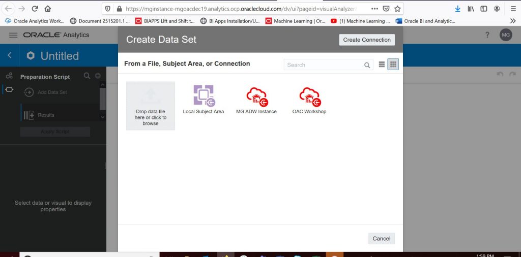
Next, we will change House ID to be treated as an attribute and not a measure so we can report against it.  After initially uploading your file, simply click on the House ID column and then, on the left-hand side where it says ‘Treat As’, change the value to attribute.  Then click ‘Add’ to add the file as a data set.

At this point, the Boston housing data set is available to be used as a training data set for our machine learning predictive model.

Step 2: Train the machine learning predictive model using the Boston housing dataset

To train the ML model in OAC we need to create a data flow.  So click on the ‘Create button’ in the upper right-hand corner and then click ‘Data Flow’.  You will be presented with a screen that asks you to pick a data set to be used by the data flow.  Please pick the Boston housing data set that you just uploaded.  After selecting your uploaded Boston housing data set, you will be presented with a screen like the one below:

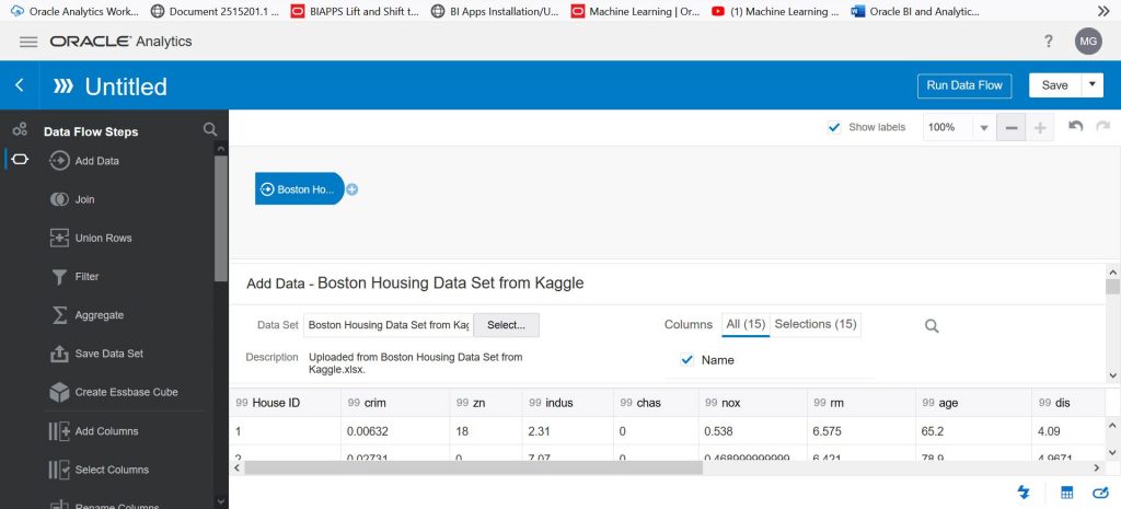
Now it is time to select the model that we will train.  Use the scroll bar on the left to scroll down to see the options available for machine learning models.  Click on ‘Train Numeric Prediction’ and drag it next to the blue ‘Boston Housing’ data set symbol.  You will see a green plus sign and then you will get the screen below:

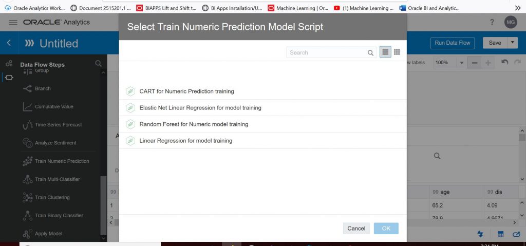
Let’s select ‘Linear Regression for model training’.  Click OK.

Guide to Oracle Cloud: 5 Steps to Ensure a Successful Move to the Cloud

Explore key considerations, integrating the cloud with legacy applications and challenges of current cloud implementations.

Get the Guide

The next step is important. This is where we pick the target column which is the column we want to predict. Click on ‘Select a column’ next to ‘Target’. Select ‘medv’ from the columns displayed. ‘medv’ stands for ‘Median Value’ and this is the value we want to predict. For the other parameters, you can leave the default values. As you scroll down you will see the value called ‘Train Partition Percent’ has defaulted to 80. This is very common and means that 80% of the data in the Boston housing data set will be used to train the model. The remaining 20% will be used to test the model (i.e., in terms of predicting housing prices).

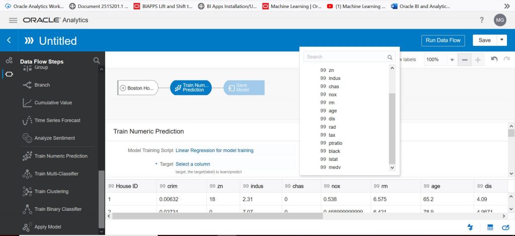
Next, we will click on the ‘Save Model’ symbol in the data flow.  We will be prompted to give the model a name.  Please call the model whatever you like.  Next, we need to save the data flow before we can run it to train the model.  Click on ‘Save’ in the upper right-hand corner and give the data flow whatever name you like.  Then click on ‘Run Data Flow’ (which is right next to ‘Save’) to train the model and to create a model that can then be applied to other data sets.  To see the model that you just created, click on the ‘hamburger’ in the upper left corner and select Machine Learning from the drop-down.  I called my model “Numeric prediction model based on the Boston housing data set’.

Step 3: Review the trained numeric prediction model.  Analyze the key drivers

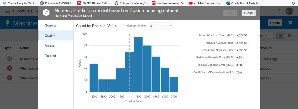
On the screen above, select your model and go to the right-hand side.  You will see an ‘Actions menu’ appear.  Click on the ‘Actions menu’ and select ‘Inspect’ to evaluate the model.  You will see the following screen:

Select ‘Quality’ to analyze the accuracy of the model.  On the screen below, we see that the Coefficient of Determination or R Squared is 70% which is generally considered good.

Now let’s take a look at what the main drivers are for the prediction of housing prices according to this model.  Click on ‘Related’ to get the screen below:

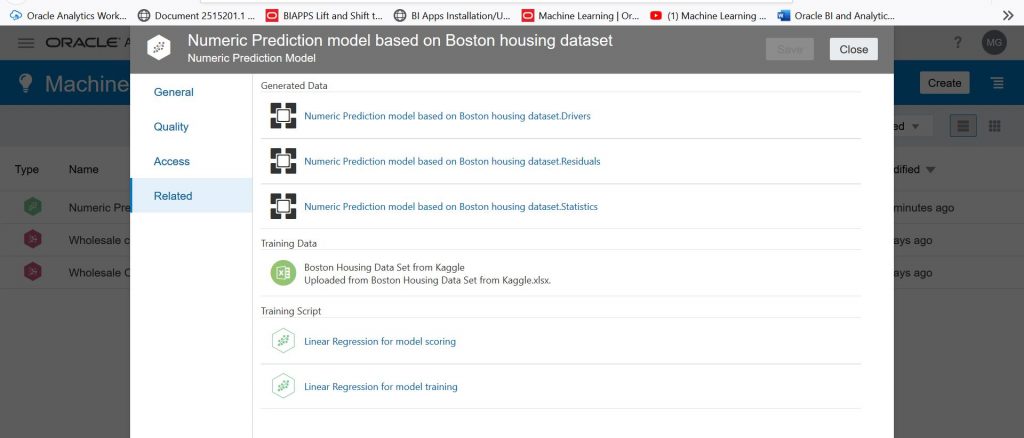
On the screen above, we will click on the first set of generated data called the “Numeric Prediction model based on the Boston housing dataset. Drivers”.  That will bring up the data set generated by the model creation process that outlines the main drivers.  Click on ‘Visualize’ in the top right-hand corner to analyze the data.  Hold down CTRL and select ‘Driver Name’, ‘Coefficient’ and ‘Correlation’ and drag them onto the visualization canvas.  If you select a visualization type of vertical bar chart, you will see the following main drivers (sorted by Coefficient high to low):

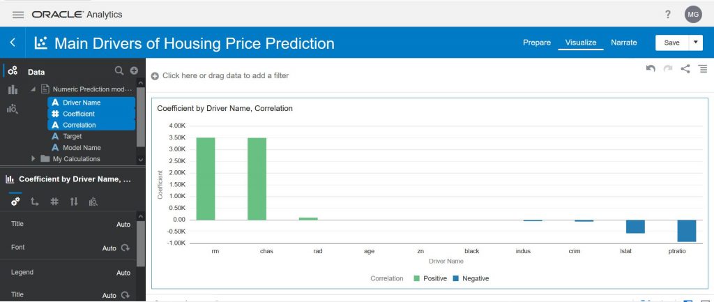
The number of rooms (rm) and whether the house is on the Charles River or not (chas) are strongly positively correlated with the housing price (as these go up so does the price of the house).  On the other side, we can see that the pupil-teacher ratio (ptratio) and % of the population of lower status (lstat) are negatively correlated with housing prices.

Step 4: Apply the machine learning predictive model we just trained to a data set to predict housing prices

Now we are ready to apply our trained ML model to predict housing prices. One thing to keep in mind is that the data set to which the ML model will be applied needs to have the same inputs (i.e., columns) as the trained ML model. To achieve this, we will apply our trained ML model to the original Boston housing data set.

To apply an ML model we need to create a data flow in OAC.  Click on ‘Create’ in the upper right-hand corner and then click on ‘Data Flow’.  Click on your Boston housing data set to add it to the data flow:

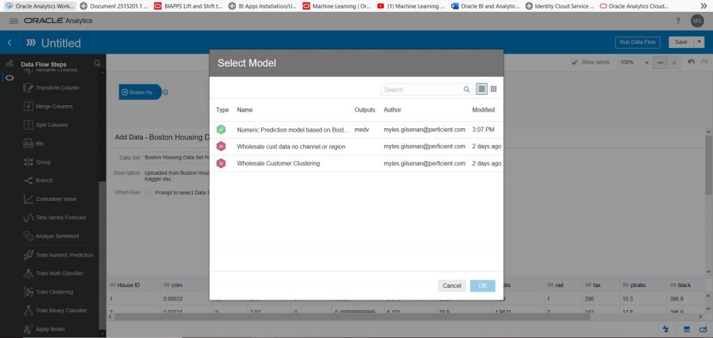
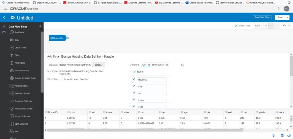Use the scroll bar on the left-hand side to scroll down until you see the ‘Apply Model’.  Drag ‘Apply Model’ onto the plus sign to the right of the Boston Housing data set.  Select the machine learning model we just created and trained (in my case it will be the model called “Numeric Prediction model based on the Boston Housing data set).  Select OK.

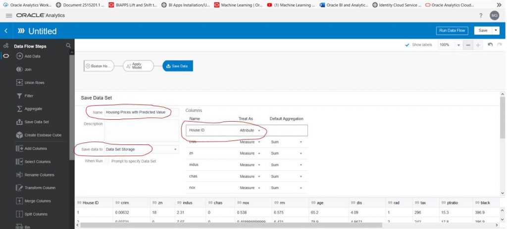
Now we need to give the column that will contain the predicted value a name and also save the data set that will be created when we run the model.  The column name for the predicted value defaults to “PredictedValue” and we will leave it that way.  Use the scroll bar on the left to scroll back up until you see ‘Save Data Set’.  Drag ‘Save Data Set’ next to the ‘Apply Model’.  Give the new data set a name, save it to data set storage and change House ID to be treated as an attribute.

Lastly, we need to save the data flow and then run it to create the new data set with the predicted value.  As we did before, please click on ‘Save’ in the upper right-hand corner and give the data flow whatever name you like. Then click on ‘Run Data Flow’ to apply the model to the Boston housing data set to predict housing prices. This will create a data set that we will analyze in the next step.

Step 5: Analyze the predicted values

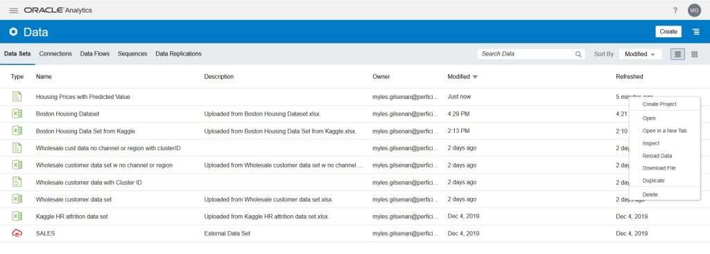
Click on the ‘hamburger’ icon in the upper left-hand corner and then click on ‘Data’ to find your data set with the predicted value.  Once you find your data set, click on the ‘Actions Menu’ for your data set and select ‘Create Project’ (my data set is called ‘Housing Prices with Predicted Value’):

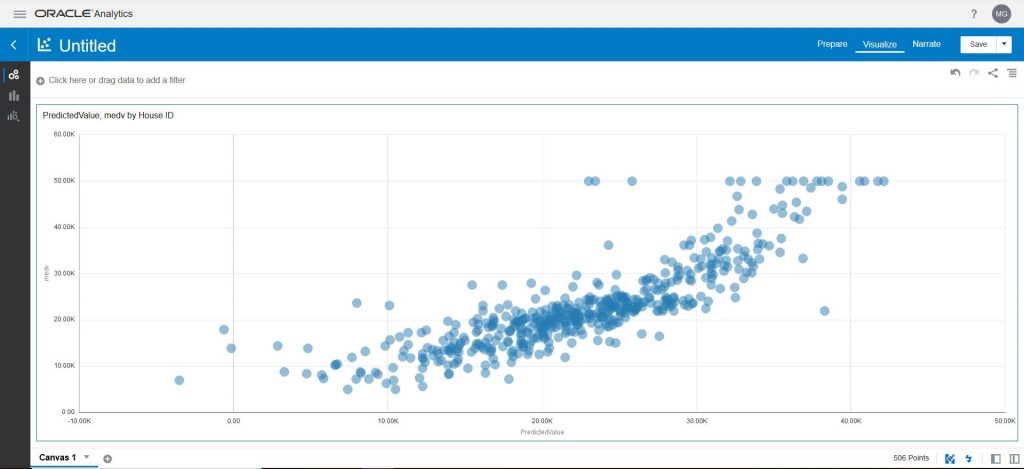
Select ‘PredictedValue’, ‘medv’ and ‘House ID’ and select ‘Scatter’ as the visualization type.  You will see the predicted value for each House ID compared to the original median value.  Although there are some outliers the majority of the predictions are close to the original house value:

I encourage you to explore the machine learning capabilities of Oracle Analytics Cloud.  Have fun!