The discovering of relationships within data (between fields) is an important part of any data mining project (in the Crisp-DM methodology, this is described as part of the “Data Understanding” stage).
This “relationship discovery” is part of developing a predictive model but is also helpful in answering specific business questions -perhaps even what originally motivated the project!
Typically, relationships between the target and the predictors are investigated (you want to see which fields are strongly associated with your target and which fields are not) and the methods used for examining relationships (between fields) depend on the “measurement levels” defined for the fields in question (I’ve debated the concept of measurement levels in previous posts and plenty of information is available online on this topic if you’re interested).
Modeler Nodes
In IBM SPSS Modeler, you use “nodes” to find relationships between fields in your data once you determine the type (categorical or continuous) of the fields.
- Two categorical fields? – use the Matrix and Distribution nodes
- A categorical and a continuous field? – Use the Means or Histogram node
- Two continuous fields? – Use the Statistics or Plot node
Some Illustrations
Two Categorical Fields
Suppose you want to explore the relationship between students who are athletes and graduate on time (two categorical fields you may recognize from some of my earlier posts). Typically, this output is expressed by cross tabulation – showing both counts and percentages.
If we use the variable file source node to absorb our data file into a stream, we can then use the Matrix and Distribution nodes to review our data (the Matrix node is used to generate the cross tabulation output and then the Distribution node is used to generate the graphical distribution graph).
A “couple of clicks and checks” on these nodes and we have some quick results – a matrix generated cross tabulation and a distribution generated graph:
Relating a Categorical and a Continuous Field
The relationship between a categorical field and a con tinuous field can be explored by comparing the means (on the continuous field) for the various categories (of the categorical field) – typically supporting the findings with a graphical display.
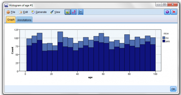
For this exercise, Santa and I wanted to determine if there was a relationship between the fields “naughty or nice” (categorical) and “age” (continuous). Again, with a few clicks of my mouse, the SPSS means node determined that age was unimportant (no relationship to) the naughty or nice field and the histogram node provided a graphical display by age group.
Relating two continuous fields
When investigating relationships between continuous fields, correlation is commonly used (correlation measures the extent to which two continuous fields are associated, that is the degree to which the relationship between two fields can be described by a straight line).
The correlation coefficient ranges from -1 to +1, where +1 represents a perfect positive linear relationship (as one field increases the other field also increases at a constant rate), and -1 represents a perfect negative relationship (as one field increases the other decreases at a constant rate). A value of zero represents no linear relationship between the two fields.
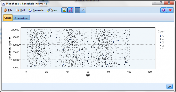
In this example, a survey file contains various continuous fields – including age and household income and I want to know the relationship between the age of the survey participant and his or her household income.
The SPSS Statistics node allows the selection of the fields (age and household income as the fields to examine as well as which statistics (such as Min, Max, Mean, Standard Deviation, etc.) to calculate and display. I my example, SPSS determined that the correlation between age and household income (based upon this file) is weak (strong and weak are words used to describe correlation. If there is strong correlation, then the points are all close together. If there is weak correlation, then the points are all spread apart).
Conclusion
I hope these simple exercises help illustrate the power of IBM SPSS Modeler. With modeler (and some reasonable data) you can predict with confidence what will happen next so that you can make smarter decisions, solve problems and improve outcomes.


