Series: Enterprise GenAI & RAG Architecture — Part 2 of 5
The Foundation Everything Else Depends On
In Part 1, we explained what RAG is and why it matters for enterprises. Now we’ll look at the technical foundation that makes effective retrieval possible: the ingestion pipeline.
Before a RAG system can answer a single question, it must go through a four-stage ingestion pipeline: Extract → Chunk → Embed → Store.
Each stage influences how accurately and efficiently the system retrieves relevant information. A well-designed ingestion pipeline improves retrieval quality and gives the LLM stronger context for generating useful answers. When ingestion falls short, even a highly capable model may struggle to produce consistently reliable results.
The most common reason enterprise RAG fails in production is poor chunking and ingestion, rather than the LLM itself.
Stage 1: Data Extraction — Getting Documents into the System
Enterprise data lives in many places. Your ingestion pipeline needs to reach all of them:
| Data Source | Extraction Method / Library |
| SharePoint / Microsoft 365 | Microsoft Graph API — ms-graph Python SDK |
| Websites / Web Pages | BeautifulSoup, Scrapy — extract and clean HTML |
| PDF Documents | PyMuPDF (fitz) or pdfminer.six — extract raw text |
| Word Documents (docx) | python-docx — preserve structure and headings |
| Jira Tickets | Jira REST API — extract titles, descriptions, comments |
| Azure DevOps (ADO) | azure-devops Python SDK — work items, wikis |
Cleaning and Normalizing
Raw extracted text is messy. Before chunking, always clean it:
- Remove HTML tags, navigation menus, cookie banners
- Fix encoding issues — normalize everything to UTF-8
- Strip page numbers, headers, footers from PDFs
- Remove duplicate documents — same content from multiple sources
- Normalize whitespace and line breaks
Skipping the cleaning step is the fastest way to pollute your vector database with noise that degrades retrieval quality.
Stage 2: Chunking — Splitting Documents into Meaningful Pieces
LLMs and embedding models have strict token limits. A 50-page PDF cannot be embedded as one unit. Chunking breaks documents into smaller, semantically coherent pieces that can be individually embedded and retrieved.
Chunking Strategies Compared
| Strategy | How It Works | Best Used When |
| Fixed-Size Chunks | Split every N tokens regardless of content | Simple pipelines, quick setup |
| Sentence Chunks | Split on sentence boundaries | Conversational content, FAQs |
| Semantic Chunks | Group sentences by topic using embeddings | Long documents, best quality |
| Recursive Split | Try paragraphs → sentences → words in order | General-purpose (recommended default) |
The Overlap Strategy — Why It Matters
Imagine a critical sentence sitting right at the boundary of two chunks. Without overlap, that sentence gets split and its context is lost in both chunks.
Overlap solves this by making each chunk share tokens with its neighbours:
Chunk 1:  [token 1 ............. token 512]

Chunk 2:              [token 463 ........... token 975]

Overlap:              [token 463 .. 512]  <-- shared context
Recommended settings: 512 tokens per chunk, 50-token overlap (≈10%)
| Chunk Size | Effect |
| Too small (< 128 tokens) | Chunks lose context — retrieval returns fragments, not answers |
| Too large (> 1024 tokens) | Irrelevant content retrieved, wastes expensive LLM tokens |
| 256–512 tokens (sweet spot) | Semantic coherence maintained, retrieval stays precise |
Tools: LangChain RecursiveCharacterTextSplitter, LlamaIndex node parsers, custom Python logic
Stage 3: Embeddings — Converting Text into Searchable Vectors
An embedding is a list of numbers that encodes the semantic meaning of a piece of text. The closer two vectors are in mathematical space, the more similar their meaning.
Example: ‘annual leave entitlement’ and ‘how many vacation days do I get?’ will produce very similar vectors — even though they share no words. This is what makes semantic search so powerful.
How Embedding Generation Works
- Each text chunk is passed to an embedding model
- The model outputs a vector — e.g. [0.23, -0.87, 0.41, … 1536 numbers]
- This vector is stored alongside the chunk text and its metadata
- At query time, the user’s question is embedded using the SAME model
- Cosine similarity between query vector and stored vectors finds the best matches
CRITICAL: The same embedding model used at indexing time MUST be used at query time. Switching models require complete re-indexing of all chunks.
Embedding Models by Cloud
| Cloud Platform | Embedding Model | Vector Dimensions |
| Azure | text-embedding-3-small / text-embedding-3-large | 1536 / 3072 |
| AWS | Amazon Titan Embeddings V2 | 1024 |
| OCI (Oracle Cloud) | OCI Embed Models (Cohere embed-english-v3.0) | 1024 |
Higher dimensions generally mean better semantic capture — but also higher storage cost and slightly slower search. For most enterprise use cases, 1024–1536 dimensions is the sweet spot.
Stage 4: Vector Databases — The Brain Behind Retrieval
A vector database stores your embedded chunks and enables fast similarity search at scale. When a user asks a question, the vector DB returns the Top-K most semantically similar chunks in milliseconds — even across millions of documents.
What Gets Stored in the Vector Database
{

  'chunk_id':   'hr_policy_001_chunk_003',

  'text':       'Employees are entitled to 20 days annual leave per year...',

  'embedding':  [0.23, -0.87, 0.41, ... ],  // 1536 numbers

  'metadata': {

    'source':   'HR_Policy_2024.pdf',

    'page':     3,

    'date':     '2024-01-15',

    'category': 'HR'

  }

}
How Similarity Search Works (ANN Search)
The vector DB uses an Approximate Nearest Neighbour (ANN) algorithm — typically HNSW (Hierarchical Navigable Small World) to find the closest vectors without scanning every single entry. This is what makes it millisecond-fast even at millions of chunks.
Vector Database Comparison Across Clouds
| Feature | Azure AI Search | AWS OpenSearch | OCI Vector Search (DB 23ai) |
| Search Type | Hybrid: BM25 + Vector + Semantic Ranker | k-NN Vector Plugin | SQL-native VECTOR type |
| Index Algorithm | HNSW + Microsoft Semantic Ranker | HNSW via k-NN plugin | IVF / HNSW in Oracle DB |
| Metadata Filtering | Rich filter expressions | Boolean + field filters | Full SQL WHERE clauses |
| LLM Integration | Native Azure OpenAI connector | Native Amazon Bedrock | Native OCI GenAI Service |
| Unique Advantage | Best hybrid search (keyword + semantic) | Widest model choice | No separate DB needed |
Azure AI Search’s hybrid mode (BM25 + vector + semantic ranker) consistently outperforms pure vector search for enterprise content — especially for technical documentation and policy documents.
Putting It All Together — The Full Ingestion Flow
Here is the complete flow from raw document to queryable knowledge:
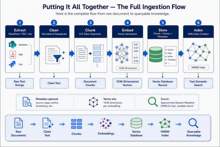
| Stage | Input → Output |
| 1. Extract | SharePoint / PDF / Jira → Raw text strings |
| 2. Clean | Raw text → Normalized, deduplicated text |
| 3. Chunk | Full document text → List of 512-token chunks |
| 4. Embed | Each chunk text → 1536-dimensional vector |
| 5. Store | Chunk + vector + metadata → Vector database record |
| 6. Index | All vectors → HNSW ANN index built for fast search |
This entire pipeline runs whenever new documents are added or existing ones are updated. In production, it’s typically triggered automatically — by a file upload, a Jira update, or a scheduled job.
➡ In Part 3, we’ll go hands-on with the Azure implementation — showing exactly how Azure Functions, Azure OpenAI, Azure AI Search, and Azure DevOps work together to build a production RAG system.