Computational Complexity Theory

Computational complexity studies the efficiency of algorithms. It helps classify the algorithm in terms of time and space to identify the amount of computing resources needed to solve a problem. The Big Ω, and Big θ notations are used to describe the asymptotic behavior of an algorithm as a function of the input size. In computer science, computational complexity theory is fundamental to understanding the limits of how efficiently an algorithm can be computed.

This paper seeks to determine when an algorithm provides solvable solutions in a short com- putational time and to find those that generate solutions with long computational times that can be categorized as intractable or unsolvable, using these polynomial functions as a classical repre- sentation of computational complexity. Some mathematical notations to represent computational complexity, its mathematical definition from the perspective of function theory and predicate cal- culus, as well as complexity classes and their main characteristics to find polynomial functions will be explained. Mathematical expressions can explain the time behavior of a function and show the computational complexity. In a nutshell, we can compare the behavior of an algorithm over time with a mathematical function such as f (n), f (n²), etc.

In logic and algorithms, there has always been a search for how to measure execution time, calculate the computational time to store data, determine whether an algorithm generates a cost or a benefit in solving a problem, or design algorithms that generate a viable solution.

Asymptotic notations

What is it?

Asymptotic notation describes how an algorithm behaves over time, when its arguments tend to a specific limit, usually when they grow very large (tend to infinity). It is mainly used in the analysis of algorithms to show their efficiency and performance, especially in terms of execution time or memory usage as the size of the input data increases.

The asymptotic notation represents the behavior of an algorithm over time by making a com- parison with mathematical functions. The algorithm has a cycle while repeating different actions until a condition is fulfilled, it can be said that this algorithm has a behavior similar to a linear function, but if it has another cycle within the one already mentioned, it can be compared to a quadratic function.

How is an asymptotic notation represented?

Asymptotic notations can be expressed in 3 ways:

• O(n): The term ‘Big O’ or BigO refers to an upper limit on the execution time of an algorithm. It is used to describe the worst-case It is used to describe the worst-case scenario. For example, if an algorithm is O(n²) in the worst-case scenario, its execution time will increase proportionally to n² where the n is the input size.
• Ω(n): The ‘Big Ω’ or BigΩ, describes a minimum limit on the execution time of an algorithm and is used to describe the best-case scenario. The algorithm has the behavior of Ω(n), which means that in the best case, the execution time of the algorithm will grow at least proportionally a n.
• Θ(n): ‘Big Θ’ or BigΘ, are to both an upper and a lower bound of the time behavior of an algorithm. It is used to explain that, regardless of the case, the execution time of the algorithm increases proportionally to the specified value. For example, if an algorithm is Θ(nlogn), your execution time will increase proportionally to nlogn at both ends.

In a nutshell, asymptotic notation is a mathematical representation of computational com- plexity expressed in terms of computational complexity. Now, if we express in polynomial terms an asymptotic notation, it allows us to see how the computational cost increases as a reference variable increases. For example, let’s evaluate a polynomial function f (n) = n + 7 to conclude that this function has a linear growth. Compare this linear function with a second one given what g(n) = n³ − 2, the function g(h) will have a cubic growth when n is larger.

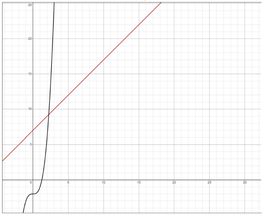
Figure 1: f (n) = n + 7 vs g(n) = n³ − 2

From a mathematical point of view, it can be stated that:

The function f (n) = O(n) and that the function g(n) = O(n³)

Computational complexity types

Finding an algorithm that solves a problem efficiently is crucial in analyzing algorithms. To achieve this we must be able to express the algorithm’s behavior in functions, for example, if we can express the algorithm as the polynomial f (n) function, a polynomial time can be set to determine the algorithmic efficiency. In general, a good design of an algorithm depends on whether it runs in polynomial time or less.

Frequency counter and arithmetic sum and bounding rules

To express an algorithm as a mathematical function and know it is execution time, it is neces- sary to find an algebraic expression that represents the number of executions or instructions of the algorithm. The frequency counter is a polynomial representation that has been worked on throughout the topic of computational complexity. with some simple examples in Csharp on how to calculate the computational complexity of some algorithms. Use the Big O, because expresses computational complexity in the worst-case scenario.

Computational complexity Constant

Analyze the function that adds 2 numbers and returns the result of the sum:

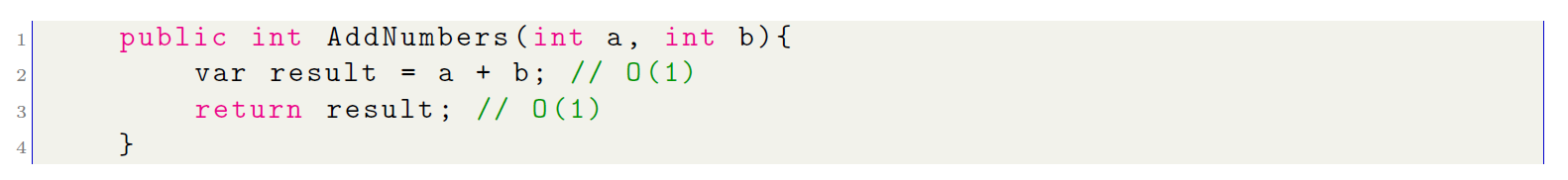
With the Big O notation for each of the instructions in the above algorithm, the number of times each line of code is executed can be determined. In this case, each line is executed only once. Now, to determine the computational complexity or the Big O of this algorithm, the complexity for each of the instructions must be summed up:

O(1) + O(1) = O(2)

The constant value is equal 2, the polynomial time of the algorithm is constant, i.e. O(1).

Polynomial Computational Complexity

Now let’s look at another example with a slightly more complex algorithm. We need to traverse an array containing the numbers from 1 to 100 and the total sum of the whole array is required:

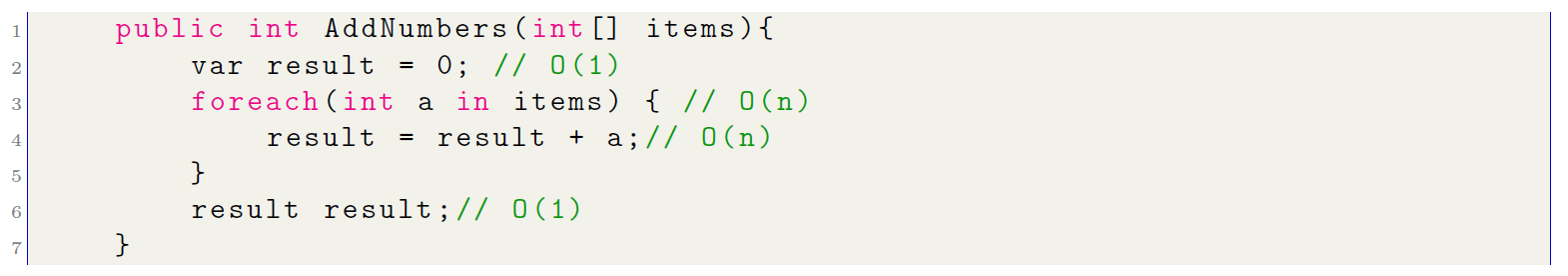
In the sequence of the algorithm, lines 2 and 6 are executed only once, but lines 3 and 4 will be repeated n times, until reaching 100 iterations (n = 100 the size of the array), to calculate the computational cost of this algorithm, the following is done:

O(1) + O(n) + O(n) + O(1) = O(2n + 2)

From this result, it can be stated that the algorithm is executed in time lineal given that O(2n + 2) ≈ O(n). Let’s analyze another algorithm, similar but with two cycles one after the other. These algo- rithms are those whose execution time depends on two variables, n and m, linearly. This indicates that the length of the algorithm is proportional to the sum of the sizes of two independent inputs. The computational complexity for this type of algorithm is O(n + m).

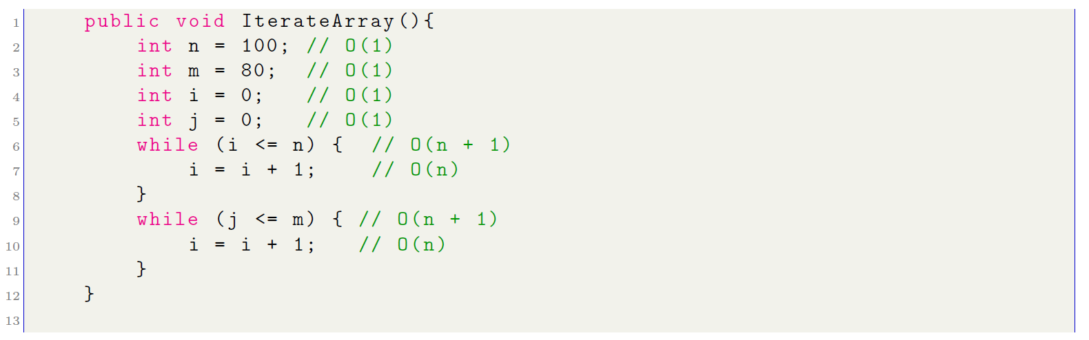
In this algorithm, the two cycles are independent since the first while represents n + 1 times while the second while represents m + 1, being n ̸= m. Therefore, the computational cost is given by:

O(7) + O(2n) + O(2m) ≈ O(n + m)

Exponential computational complexity

For the third example, the computational cost for an algorithm containing nested cycles is analyzed:

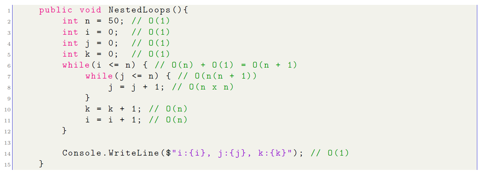
The conditions in a while (while) and do-while (do while) cycles are executed n + 1 times, as compared to a foreach cycle. These loops do one additional step: validate the condition to end the loop. In line number 7, by repeating n times and doing its corresponding validation, the computational complexity at this point is n(n + 1). In the end, the result of the computational complexity of this algorithm would result in the following:

O(6) + O(4n) + O(2n²) = O(2n² + 4n + 6) ≈ O(n²)

Logarithmic computational complexity

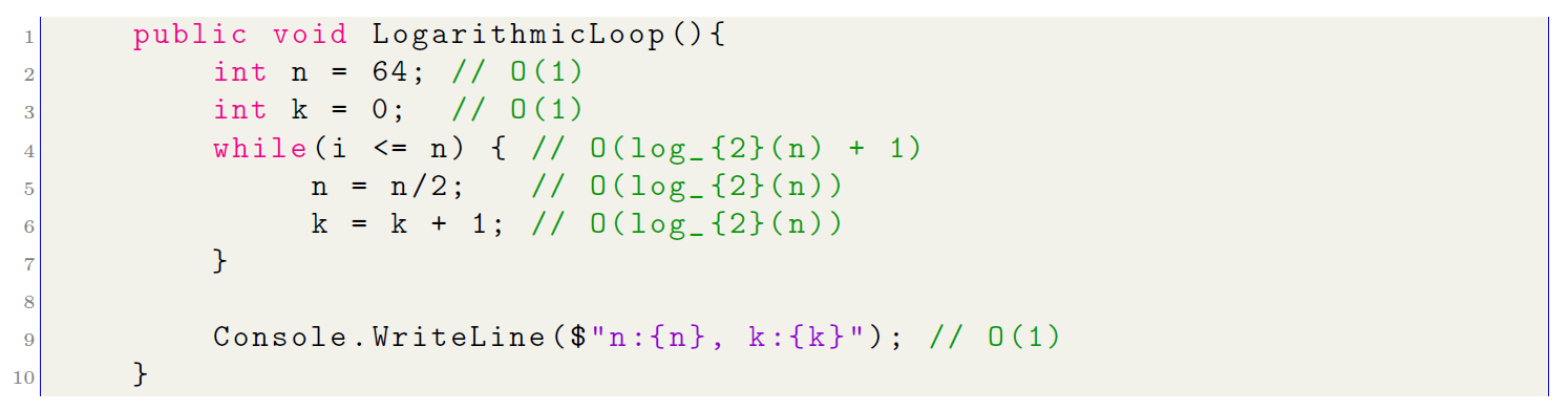
• Logarithmic Complexity in base 2 (log₂(n)): Algorithms with logarithmic complexity O(logn) grow very slowly compared to other complexity types such as O(n) or O(n²). Even for large inputs, the number of trades does not increase Let us analyze the following algorithm:

Using a table, let us analyze the step-by-step execution of the algorithm proposed above:

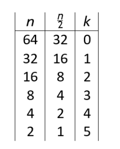
Table 1: Logarithmic loop algorithm execution

If you examine the sequence in Table reftab:tab1, you can see that their behavior has a logarithmic correlation. A logarithm is the power that must be raised to get another number. For example, log₁₀100 = 2 because 10² = 100. Therefore, it is clear that the base 2 must be used for the proposed algorithm:

64/2 = 32

32/2 = 16

16/2 = 8

8/2 = 4

4/2 = 2

2/2 = 1

It can be calculated that log₂64 = 6, which means that the six (6) loop has been executed six (6) times (i.e. when k takes values {0, 1, 2, 3, 4, 5}). This conclusion confirms that the while loop of this algorithm is log₂(n), and the computational cost is shown as:

O(1) + O(1) + O(log₂(n) + 1) + O(log₂(n)) + O(log₂(n)) + O(1)

= O(4) + O(3log₂(n))

O(4) + O(3log₂(n)) ≈ O(log₂(n))

• Logarithmic complexity (nlog(n)): Algorithms O(nlog(n)) have an execution time that increases in proportion to the product of the input size n and the logarithm of n. This indicates that the execution time does not double if the input size is doubled, on the contrary, it increases less significantly due to the logarithmic factor. This type of complexity has a lower efficiency than O(n²) but higher than O(n).

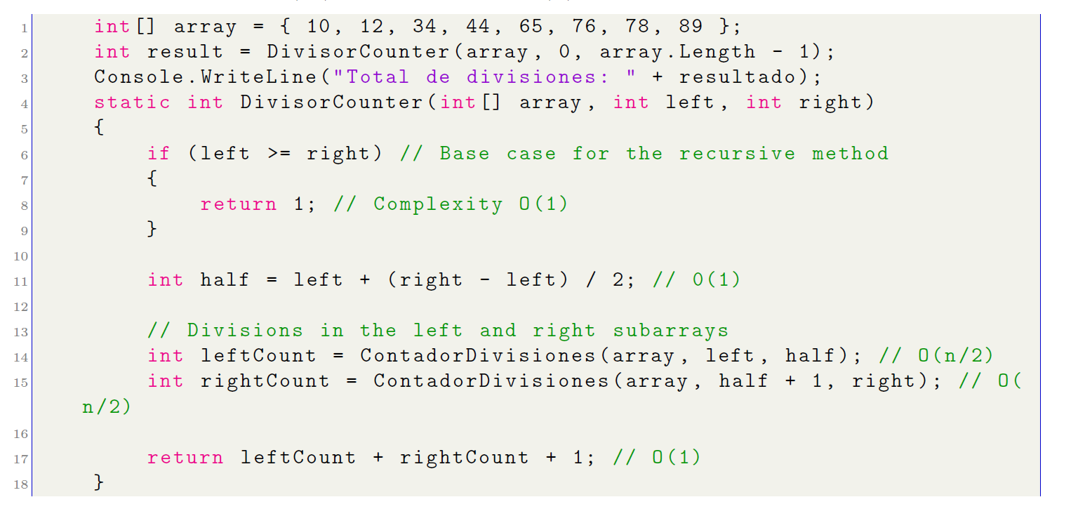
O(2 ∗ (n/2)) + O(1) ≈ O(nlog(n))

Analyzing the algorithm proposed above, mentioning the merge sort algorithm, the algorithm performs a similar division, but instead of sorting elements, it counts the possible divisions into subgroups. The complexity of this algorithm is O(nlog(n)) due to recursion and n operations are performed at each recursion level until the base case is reached.

Finally, in a summary graph, you can see, the behavior of the number of operations performed by the functions based on their computational complexity.

Example

An integration service is periodically executed to retrieve customer IDs associated with four or more companies registered with a parent company. The process performs individual queries for each company, accessing various databases that use different persistence technologies. As a result, an array of data containing the customer IDs is generated without checking or removing possible duplicates.

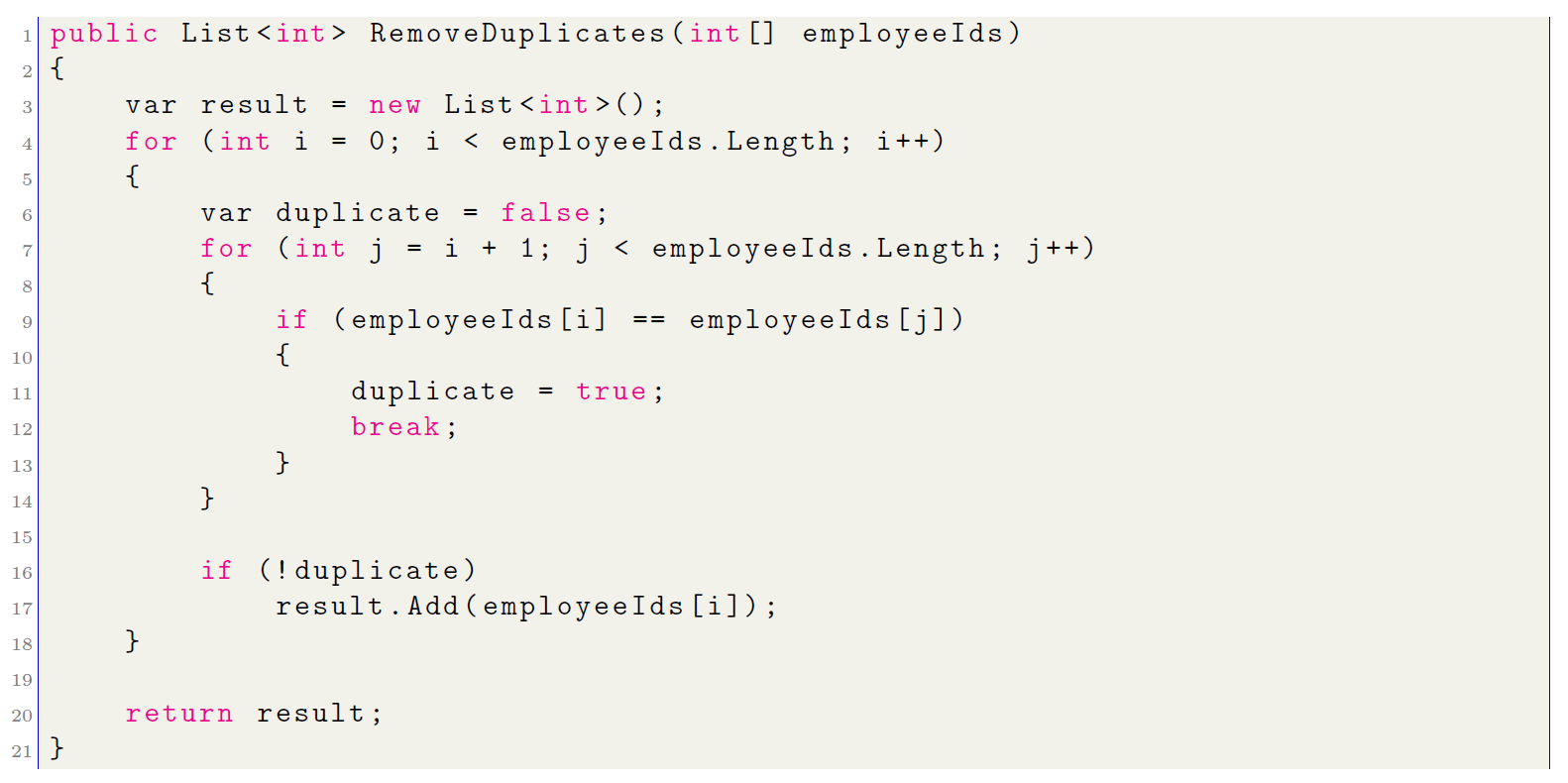
In this case, the initial approach would involve comparing each employee ID with all other elements in the array, resulting in a quadratic number of comparisons, i.e., O(n²):

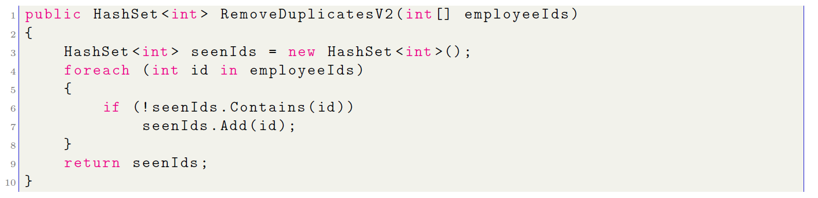
In a code review, the author of this algorithm will be advised to optimize the current approach due to its inefficiency. To solve the problems related to nested loops, a more efficient approach can be taken by using a HashSet. Here is how to use this object to improve performance, reducing complexity from O(n²) to O(n):

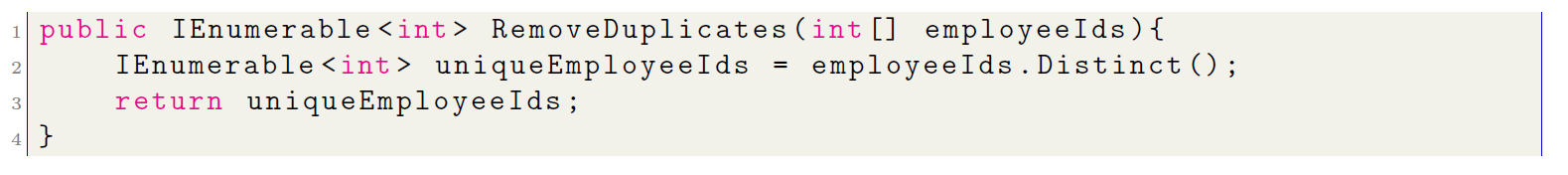
Currently, in C# you can use an object called IEnumerable, which allows you to perform the same task in a single line of code. But in this approach, several clarifications must be made:

• Previously, it was noted that a single line of code can be interpreted as having O(1) complex- ity. In this case, it is different because the Distinct function traverses the original collection and returns a new sequence containing only the unique elements, removing any duplicates using a HashSet, which, as mentioned earlier, results in O(n) complexity.
• The HashSet also has a drawback: in the worst case, when collisions are frequent, the complexity can degrade to O(n²). However, this is extremely rare and typically depends on the quality of the hash function and the characteristics of the data in the collection.

The correct approach should be:

Conclusions

In general, we can reach three important conclusions about computational complexity.

• To evaluate and compare the efficiency of various algorithms, computational complexity is essential. Helps to understand how the execution time or resource usage (such as memory) of an algorithm increases with input size. This analysis is essential for choosing the most appropriate algorithm for a particular problem, especially when working with significant amounts of data.
• Algorithms with lower computational complexity can improve system performance signifi- cantly. For example, the choice of an algorithm O(nlogn) instead of one O(n2) can have a significant impact on the amount of time required to process large amounts of data. Ef- ficient algorithms are essential to ensure that the system is fast and scalable in real-world applications such as search engines, image processing, and big data analytics.

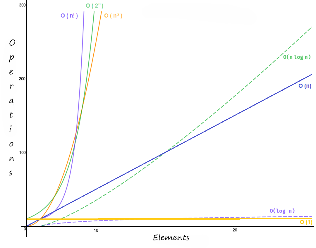
Figure 2: Operation vs Elements

• Understanding computational complexity helps developers and data scientists to design and optimize algorithms. It allows for finding bottlenecks and performance improvements. By adapting the algorithm design to the specific needs of the problem and the constraints of the execution environment, computational complexity analysis allows informed trade-offs between execution time and the use of other resources, such as memory.

References

• Roberto Flórez Algoritmia Básica, Second Edition, Universidad de Antioquia, 2011.
• Thomas Mailund. Introduction to Computational Thinking: Problem Solving, Algorithms, Data Structures, and More, Apress, 2021.