Spark optimization techniques

Spark has been referred to as a “general purpose distributed data processing engine” and “a lightning fast unified analytics engine”.

With its simple APIs, it simplifies the lives of developers and programmers. It is capable of handling upto petabytes of data and manages thousands of virtual or physical machines all at once.

The Apache Spark framework is one of the most popular cluster computing frameworks for handling big data. However, while running complex spark tasks, taking care of the performance is equally important.

Apache Spark optimization improves in-memory computations and increase efficiency of jobs for better performance characteristics, depending on data distribution and workload.

Some of the basic spark techniques you can adapt for greater performance include

• Cache and Persist
• Shuffle Partitions
• Broadcast Join strategy
• File format selection

Cache and Persist

The highly efficient and parallelized execution has a cost: it is not easy to understand what is happening at each stage. You have to collect the data, or a subset of it, to a single machine in order to view it after some transformations.

So Spark have to determine the computation graph, optimise it, and carry out this activity. This could take a long time if your dataset is large.

This is particularly time-consuming, if caching is disabled and Spark have to read the input data from a distant source, like a database cluster or cloud object storage like S3.

Spark has its own caching mechanisms, such as persist() and cache().The dataset will be stored in memory using cache() and persist().When you have a small dataset that needs to be used repeatedly in your program, we cache it.

Cache():-  Always in Memory

Persist():-  Memory and disk

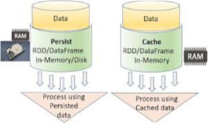
If you have a limited dataset that is utilised multiple times in your program, persist and cache mechanisms will store the data set into memory whenever there is a need.

Applying df.Cache() will always store the data in memory, whereas applying df.Persist() will allow us to store some data in memory and some on the disk.

For Example:-

I had taken a sample data and load it as dataframe.

Then I apply simple action such as count on it. It took approx 7 sec.

Choosing a Global Software Development Partner to Accelerate Your Digital Strategy

To be successful and outpace the competition, you need a software development partner that excels in exactly the type of digital projects you are now faced with accelerating, and in the most cost effective and optimized way possible.

Get the Guide

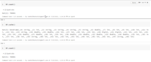
After caching,  action was done in 0.54 sec.

Suppose I run it with GB’s or TB’s of data, it will take several hours to finish. So, Knowing these basic concepts in Spark would therefore save several hours of additional computation.

Shuffle Partitions

The purpose of shuffle partitions is to shuffle data prior to joining or aggregating it. When we perform operations like group by, shuffling occurs. During shuffling, huge amount of data were transferred from one partition to another.  This can also happen across partitions that are on same machine or between partitions that are on the different machines.

When dealing with RDD, you don’t need to worry about Shuffle partitions. Suppose we are doing groupBy on an initial RDD that is distributed over 8 partitions. Despite groupBy, the partition count remains unchanged in RDD. But the case is not same with data frames.

For example:-

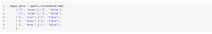
df = spark.createDataFrame(

[('1', 'true'),('2', 'false'),
('1', 'true'),('2', 'false'),
('1', 'true'),('2', 'false'),
('1', 'true'),('2', 'false'),
('1', 'true'),('2', 'false'),
])
df.rdd.getNumPartitions()
8
group_df = df.groupBy(“_1”).count()
group_df.show()
+—+—–+

| _1|count|

+—+—–+

|  1|    5|

|  2|    5|

+—+—–+
group_df.rdd.getNumPartitions()
200

The shuffle partition count in the above example was 8, but after applying a groupBy, it was increased to 200. This is so because the DataFrame’s default Spark shuffle partition is 200.

The number of spark shuffle partition can be dynamically altered with the conf method in Spark session.

sparkSession.conf.set("spark.sql.shuffle.partitions",100)

or Dynamically set during spark-submit initialization spark.sql.shuffle.partitions:100.

Choosing the appropriate shuffle partition count for your spark configuration is crucial. For example, let’s say I want to perform a groupBy on a very tiny dataset using the default shuffle partition count of 200. In this situation, I might use too many partitions and overburden my spark resources.

In a different scenario, I have very huge dataset and I ‘m running a groupBy with the default shuffle partition count. So, I might not use all of my spark resources.

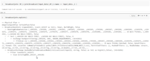
 Broadcast Join strategy

When we join two large datasets, what happens in the backend is that large amount of data get shuffled between partitions in the same cluster as well as between partitions of different executors. When we need to join a smaller dataset with a larger dataset, we perform broadcast joins. Spark broadcasts the smaller dataset to all cluster nodes when we apply a broadcast join, so the data to be joined is present on all cluster nodes and spark can do a join without any shuffling.

Using broadcast join you can avoid sending huge data over the network and shuffling. The explain method can be used to validate whether the data frame has been broadcasted or not. By default the maximum size for a table to be considered for broadcasting is 10MB.This is set using the variable such as

spark.sql.autoBroadcastjoinThreshold

. The example below illustrates how to use broadcast joins.

File Format Selection

• Spark supports a variety of formats, such as CSV, JSON, XML, PARQUET, ORC, AVRO, etc.
• Choosing parquet files with snappy compression can optimize Spark jobs for high performance and optimal analysis.
• Parquet files are native to Spark, which contain metadata along with their footers.

With Spark, you can work with a wide range of file formats, like CSV, JSON, XML, PARQUET, ORC, and AVRO. It is possible to optimize the Spark job by using a parquet file that has snappy compression. We know that a parquet file is native to spark and is in binary format. Along with the metadata, the file also carries a footer. When you create a parquet file, you’ll find  .metadata file along with the data file in the same directory. The example below shows to write parquet file for better performance.

DF = spark.read.json(“file.json”)

DF.write.parquet(“file.parquet”)

Spark optimization can be achieved in several ways, if these factors are used correctly for proper use cases. we can :-

• Get rid of the time-consuming job process.

• improve data distribution and workload.

• Manage resources so that performance can be optimized.

This post provides an overview of some of the basic aspects involved in creating efficient Spark jobs. In most cases, solving spark problems by following these techniques will resolve the issue in efficient manner.

Happy Learning!!